Scaling Law, Architecture for Stability and Layer Stacking
Scaling Law
Scaling law is one of the most important findings in LLMs (and neural networks in general) 1. You can make almost all important decisions about training of models with scaling law. For example you can choose model size, number of training steps 2, hyperparameters such as learning rate and batch size 3, learning rate schedules 4, mixture of training datasets 5, etc.
So if you are serious about builiding or understanding LLMs, you should be able to estimate the scaling law. And…I didn’t have experiences about it. Anyway you need to have nontrivial amout of computing power because estimation of scaling law requires to train many models. But again TPU Research Cloud Program (https://sites.research.google/trc/about/) allowed me to get (at least for me) interesting results. I am deeply grateful to them.
Code Base
First I needed to get simple and hackable code base for training language models in jax. But also I should support at least FSDP to training interesting sized models. I have first considered MaxText (https://github.com/google/maxtext) but I found NanoDO (https://github.com/google-deepmind/nanodo) is more simple.
NanoDO is minimal framework for training language models in jax with support of FSDP. I have modified it to support multi-host training. I have uploaded code that I have used for experiments.s (https://github.com/rosinality/nanodo, messy!)
Caveats
NanoDO uses Grain (https://github.com/google/grain) for data loading. Grain is quite similar to PyTorch dataloader, which uses multiprocessing to load data in parallel and allows arbitrary python code to preprocess data. Grain depends on ArrayRecord (https://github.com/google/array_record) which is a data format that allows random access. So it is quite trivial to restart training from previous checkpoint.
But due to support for random access, you cannot directly use GCP buckets. You should mount GCP bucket to your VM instance using gcsfuse, and you can refer to script from MaxText (https://github.com/google/maxtext/blob/main/setup_gcsfuse.sh). But…I found this is quite unstable, and other peoples also experienced this (https://github.com/google/maxtext/issues/786). Any it works well after some warmup (?) period. I don’t know how google deals with this.
Checkpointing using Orbax requires storage global, that is accessible from all hosts. Like GCP buckets. (https://github.com/google/orbax/issues/999) You can just use GCP bucket for this, but it is not documented well.
Experiment Settingsss
I made my experiment settings with reference to Resolving Discrepancies in Compute-Optimal Scaling of Language Models 6. It allowed me to do manageable sized experiments for estimating scaling law. My settings is as follows.
| Setting | Value |
|---|---|
| Sequence Length | 1024 |
| Vocabulary Size | 32101 (Llama 1) |
| Number of Heads | 4 (Small, but same with 6.) |
| FFN Activation | SwiGLU |
| FFN Multiplier | 3.5 |
| Positional Embedding | RoPE |
| Independent Weight Decay | 1e-4 |
| Attention Logit Softcapping | 50 (Adopted from Gemma 2 7) |
| Final Learning Rate Multiplier | 0.1 |
| Warmup Steps | Varying, with tokens same size with model parameters |
| Embedding Init | Normal(0.01) |
| Linear Init | Variance Scaling 1.0, fan-in |
| Residual Block Output Linear Init | Variance Scaling 1.0 / sqrt(number of layers), fan-in |
| LM Head Init | Variance Scaling 1.0, fan-in |
| Weight Tying | False |
| Normalization | RMSNorm |
| Training Dataset | FineWeb-Edu |
Final loss for each model is calculated using separate validation set. Model for each scale was like this
| ID | Parameters | FLOPS/Token | Dimensions | Layers | Batch Size | |
|---|---|---|---|---|---|---|
| 1 | 19M | 86M | 288 | 8 | 112 | |
| 2 | 24M | 116M | 320 | 9 | 128 | |
| 3 | 34M | 175M | 384 | 10 | 160 | |
| 4 | 56M | 311M | 480 | 12 | 208 | |
| 5 | 86M | 503M | 576 | 14 | 256 | |
| 6 | 110M | 652M | 640 | 15 | 320 | |
| 7 | 152M | 932M | 704 | 18 | 384 | |
| 8 | 238M | 1479M | 832 | 21 | 512 | |
| 9 | 383M | 2388M | 1024 | 23 | 640 | |
| 10 | 509M | 3195M | 1120 | 26 | 896 | |
| 11 | 691M | 4313M | 1312 | 26 | 1024 |
In 6 it is recommended to consider include number of parameters of the embedding to the model. As I have used untied embeddings, I only counted number of parameters of embeddings, not LM head. (But anyway, for estimating scaling law I have used FLOPS/token instead of parameters.)
I have adopted batch sizes from 6, but as my sequence length is half, I have double the batch sizes. Instead of using learning rate scaling law, I have used same learning rate for all models with 3e-3 which I have searched with 34M model, but I have scaled learning rate of linear weights for another models with $384 / dim$. 8 9 10 I found this transfers with different model scales.
I have used AdamW with eta_1 = 0.9$, eta_2 = 0.98$. It was my mistake to use same eta_2$ for all scales, but I expect 0.98 is close enough to optimal for this model scales.
Models trained with same FLOPS budget, 1.25e17. For larger scale integer multiple of 1.25e17 is used.
Results
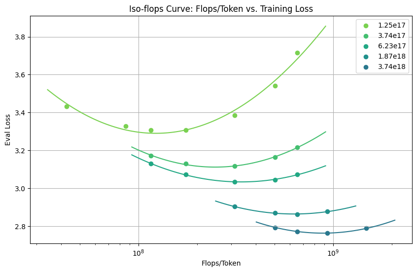
So after hyperparameter tuning and experiments I got this IsoFLOPS curve 2. I have measured FLOPS/Token instead of parameters, with reference to 2. Anyway I have suprised that I could get a such nicely fitted curve.

So by finding minimum of the IsoFLOPS curve for each training scales, I was able to get loss curve for each training scales given allocated FLOPS/Token is optimal.
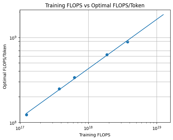
Then I drew for each training FLOPS, optimal allocation of FLOPS/Token of the model. Fitted function is $0.0149C^{0.58}$ and exponent 0.58 which is close to 0.578 that is estimated for OpenWebText2 in 3.
Architectural Modifications and Learning Rate Sensitivity
During experimentation I have touched about learning rate transfer for efficiency. After the experiment, I thought might attention logit softcapping (and z-loss 11) was vastly beneficial for learning rate transferability. It is known that explosion of attention logit induces training instabilities for higher leearning rates, and thus reduce transferability of learning rates. One of well-known solution for this phenomena is QK Norm which bounds maximum attention logits 12. So maybe softcapping of attention logits could have similar effect, as it also bounds attention logits anyway.
QK Norm is trick of applying layer normalization (or RMSNorm) on query and key before computing attention logits, like $\operatorname{LN}(Q)\operatorname{LN}(K)^\intercal$. Attention logit softcapping is applying softclipping using tanh like $\alpha\operatorname{tanh}(\frac{1}{\alpha}QK^\intercal)$, where $\alpha$ is a constant like 50. Post normalization is applying layer normalization after output linear layer for each residual block, like $y = x + \operatorname{LN}(\operatorname{Block}(x))$. Post normalization was actually refering normalization setting of original transformer paper, $y = \operatorname{LN}(x + \operatorname{Block}(x))$ 13. But it is not popular these days due to training instabilities 14 (it is commonly said that post normalization is better for performance, though 15) and many people started refer $y = x + \operatorname{LN}(\operatorname{Block}(x))$ as a post normalization 16 17.
Therefore I started learning rate sensitivity experiments, like 9. The main focus of 9 was the change of the loss given change of the learning rate, and measuring width of basin of learning rates that induces similar loss. Slightly different from this, I want to know that architectural modifications like QK Norm or Softcapping can allow learning rate transfer. Actually in 12 authors have shown that with QK Norm it is possible to use same learning rate 1e-3 for ViT-L (307M) and ViT-22B (of course, 22B)! It is more than 70x increase in model sizes. (Also, authors reported that it is not trainable in that scale without QK Norm. https://x.com/jmgilmer/status/1626276273168470016)
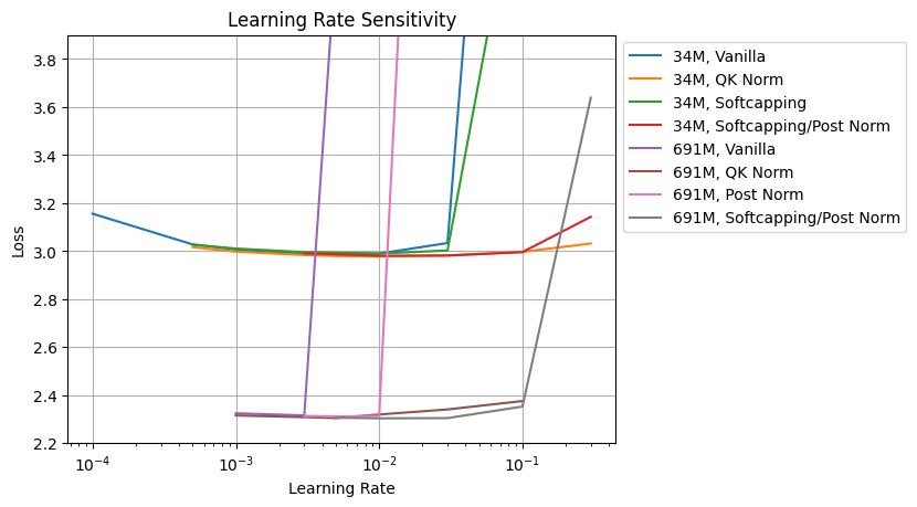
I have trained 34M and 691M models with fixed 50K steps and 5,000 warmup steps. I have used batch size described above, as I thought it is more natural settings. (increase batch sizes along with model size increases.) So batch size increasement can give additional stabilities for larger models. But, apparently, it is not enough for larger models as shown in vanilla settings.
I found Attention logit softcapping is not enough for reduce learning rate sensitivity, and is has similar curve to vanilla case. But, with post normalization (which is also used in Gemma 2), it is possible to have similar reduced sensitivity to QK norm. Again, post norm itself is not enough for stable training, as shown in 691M curves with post norm without softcapping.
Also, if comparing basin of learning rate sensitivity between 34M and 691M models, with Softcapping + Post norm or QK norm allows to use similar learning rate for both models. Apparently it is not possible with vanilla transformer. Learning rate left-shifts as model size increases.
And I constantly got a slightly better results with QK norm or Softcapping/Post Norm, about loss 0.01. Anyway it seems like that there is reason Gemma 2 (and Grok-1 https://github.com/xai-org/grok-1) have used softcapping and post norm, as it is anyway possible to train models with that sizes in vanilla settings. Recently OLMoE also reported with QK norm they can achieve better results. I think it would be similar with softcapping and post norm.
Why combination of Softcapping and Post Norm helpful?
It is known that QK norm suppresses unbounded increase of attention logits, thus stabilizes training 12 9. But as shown in softcapping only results, bounding logit value itself not sufficient to stabilize training. Maybe it is also required to modulate distribution of attention logits.
Again, post normalization is somewhat helpful for stabilize training, but it is likely that absolute clipping of attention logit is required to further stabilization. So I suspect post norm is helpful for more sane overall distribution of logits, and softcapping is helpful to bound and remove outliers of logits. (CogView 18 and Swin Transformer V2 16 reports using post normalization reduces maximum value or variance of features. Swin Transformer V2 also have used cosine similarity for attention logits, and it is reported that is makes “milder” attention logits.)

Pre Normalization and Post Normalization, or “Sandwich Norm” in CogView 18. Sandwich Norm and subtraction of maximum value to prevent overflow effectively suppresses maximum value of output embeddings.

Signal propagation plot (Average feature variance) of Swin Transformer V2. Post normalization suppresses increase of average feature variance, compared to pre normalization across all model sizes and supervised or self-supervised training.
It is well known fact that LLMs have outlier values in features 19 20 21. Even though pre normalization normalizes input features, these outliers can cause distribution shift 22 23. Post normalization can alleviate this as shown in. But it is not enough for overall training stabilization, as query and key projection can still induces outliers or large attention logits. Softcapping is helpful for this by directly suppress maximum logits.
If your tasks is more picky like autoregressive text to image generation, you may also need to bound attention logits using QK norm and also post normalization as in 17. It might be due to gating of SwiGLU in FFN, as suggested in 17.
This is mostly a kind of guesswork, surely more investigation is needed.
Do we need to increase batch size along with model size?
It is general knowledge that any batch size below “critical batch size” is okay for training of models 24. But there are puzzling papers that reported there are also minimum batch sizes for training models that if smaller than that training loss will be increased 3 6.
One thing make it hard to experiment with optimal batch sizes is that you need to adjusts many hyperparameters along with learning rates, especially Adam $\beta_1$ and $\beta_2$ 25. It will be best to grid search with this, but given compute budgets, I have manually choosed candidate hyperparameters with learning rates and $\beta_2$. (Based on simple logic - smaller $\beta_2$ will be better for small batch sizes, and larger learning rates will be better for larger batch sizes.)
Maybe it will be also needed to adjust $\beta_1$ to get optimal results. But practically it makes problem harder for actual training, as it means that you need to adjust one more hyperparameters to get a optimal result for small batch sizes. So I think adjusting learning rate and $\beta_2$ is actually more practical setting. (More practically, trying to find minimum batch sizes that works well is not important. What we want to know is largests batch sizes that works well.)
In this experiment I have trained all of the models with same training tokens 15.7B (which corresponds to 30K steps with 512 batch size.) and number of training steps will be adjusted with batch size. I have decayed learning rate to 1e-5 of peak learning rate as this affects results a lot.

And here is the results. I annotated as a optimal if loss is within 0.25% difference to optimal/minimum loss, which is similar to 3. (I think this is very important, as in many cases basins around optimal learning rate or batch size is quite flat. So if you just pick absolute minimum it could be misleading.)
So I found that maximum allowable batch sizes is increasing with model size. Also, I found that there are minimum batch sizes for each model that below of it there are training difficulties. I have found slight right-shift of optimal batch sizes with model sizes. It is hard to directly compare, but I think I found less severe than previous papers. I think candidate resons for this is 1. I have experimented only larger end of model sizes. 2. Right-shifting of batch siszes is less prominent than increase of allowable batch sizes 3. I have used fixed token budge for each model sizes, but previous papers have used chinchilla optimal scaling which increase token budgets along with model sizes. As it is common to use far more training tokens than chinchilla optimal regardless of model sizes, I think my setting could be useful for that scenario.
So why phenomena like this happens? I don’t have theoretical explanation for this. But my guess is like this:
- Larger models are instable, and they benefit more from reduced noise of larger batch sizes.
- Maybe larger models can better “utilize” informations from larger batch sizes.
- Smaller models are harder to train, and they benefit from absolute increase of training steps. (smaller batch sizes.)
As my guess was around training instabilities, I have thought that more instable models can have different patterns. As I have experimented with softcapping and post norm, I have tried to do similar experiments with vanilla transformer which could be more “instable”.
You can refer to this result from above plot with 238M Vanilla. It has reduced gaps between larger and smaller batch sizes by increased minimum loss, and has similar loss for small batch sizes. This is only partial evidence, but I think this suggests maybe there are reasons other than training stabilities for this batch size scaling phenonmena. I think more investigation will be meaningful for this problem.
Layer Stacking
Training efficiencies, especially reducing number of training tokens given the loss or performances is now one of the most important things in LLM training. One part of problem is that as sheer amount of compute is needed, just slight reduction in training tokens could result in large amount of reduction of resources. (Or you can think this as a virtual increasing factor for resources, that if you can reduce 10% of training times, it could correspond to actual increasement of number of GPUs you have https://nonint.com/2023/11/05/compute-multipliers/.) More importantly, as gathering data is bottleneck, reducing number of training tokens actually corresponds to increase of the size of the data you have. If you can reach same performance with 50% of training tokens, then it corresponds to 2x increase of total data.
There are promising approaches for this problem like RHO-Loss 26 27 28. I also found stacking transformer layers for boosting training speed is interesting 28 29. So I have tried to replicate results of 28.
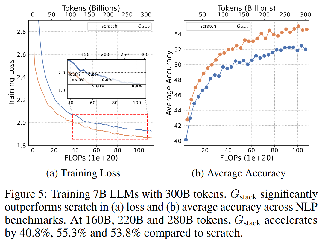
And the method is simple. You just need to stack transformer layers, like A, B, C to A, B, C, A, B, C. So I thought I can easily replicate their results, even there are some differences in training setups.

And I found that is is not an easy problem. There are many hyperparameters that governs early training dynamics like weight decay. And I found this hyperparameters can affect overall results by accelerating early trainings, but eventually at the final steps from scratch training gets better results than layer stacked models, which is worst thing can happen with training acceleration methods.
So I have experimented with more similar settings to 6, especially sequence length, learning rate, and weight decay. I got slight acceleration for layer stacking, but it was not very large at this training stage, and it will be smaller if you also consider tokens used for training small models.
I think this worth investigating, but maybe I should be cautious more on exact training settings for replication.
Weight Decays
For above experiments I have used independent weight decay of 1e-4 9 6. But after above experiments I wanted to investigate more on weight decay. Especially weight decay scheduling which appears in PaLM 11.
Scheduling weight decay is not common, and I can’t find many previous examples for this 30 31. But recently Llama 3 have reported that they have used weight decay scheduling for scaling experiments 32.
Weight decay scheduling, which appears in PaLM, is setting weight decay to proportional to learning rates, line $weight\ decay = lr^2$. Llama 3 have used $weight\ decay = 0.1 imes lr$ for scaling experiments, which would be equivalent to $weight\ decay = 0.1 \times lr^2$ in PaLM 11 as PaLM uses Adafactor 33 which uses independent weight decay in default, in contrast to PyTorch or Optax implementation of AdamW that may have been used in Llama 3 which uses coupled weight decay to learning rates.
What would be meaning of this scheduling? First, if you are using coupled weight decay than using larger learning rate also means larger weight decay, so it can hinder training. But if you are using weight decay scheduling then weight decay will be small at the final stage of training, and it could be beneficial by avoiding using too large weight decay. Also it could be useful for model performances as it would reduce regularizing effect of weight decay at the final stage thus reduce bias of the model.
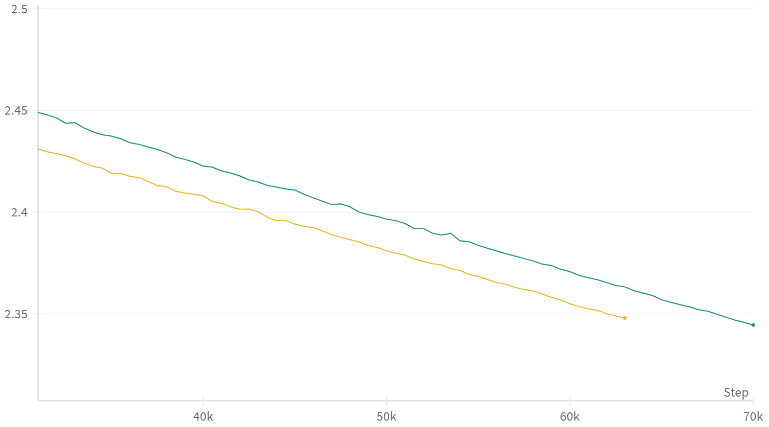
So I have experimented with various settings of weight decay. 1. PyTorch/Optax default weight decay which couples learning rate with weight decay. 2. Independent weight decay of 1e-4 which corresponds to 1e-4 / peak learning rate in PyTorch or Optax. 3. Weight decay scheduling of $weight\ decay = lr$. I have trained 724M model during 50K steps with various learning rates.
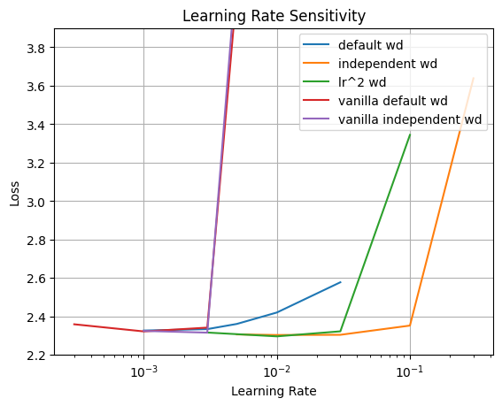
Similar with results in 9, I found that using default coupled weight decay hinders training. Using independent weight decay relieves this and widens optimal learning rate basins. (But this is not useful for vanilla transformer as it will blow-up at large learning rates anyway.) Weight decay scheduling has similar effect to independent weight decay, and it is less effective at largest learning rates than independent weight decay, but it can reach slight better loss at optimal learning ratess, potentially due to reducing bias of the model.
It is ironic that independent weight decay which decouples weight decay from learning rates, and weight decay scheduling which couples weight decay with learning rate more has similar effect on training. Practically using weight decay scheduling could be dangerous as it tends to have less weight decay if you compare with coupled weight decay, and increasing scale of it by $weight\ decay = 10 \times lr$ was not work very well. I am very interested in weight decay of actuall Llama 3 405B training.
Conclusion
Similar to previous experiments, Preliminary Explorations on UL2 and Second-order Optimizers I was able to get (at least for me) interesting results that is hard to get without large amount of computes. Thank you again for TPU Research Cloud, and I am not more falling in love with TPU.
Many things like scaling law estimation, learning rate sensitivity with architectural modifications, estimating optimal batch sizes, and investigating of layer stacking is almost direct replication efforts of previous papers. But I think softcapping and post normalization results and weight decay scheduling could be interesting to others.
Kaplan, J., McCandlish, S., Henighan, T., Brown, T. B., Chess, B., Child, R., … & Amodei, D. (2020). Scaling laws for neural language models. arXiv preprint arXiv:2001.08361. https://arxiv.org/abs/2001.08361 ↩︎
Hoffmann, J., Borgeaud, S., Mensch, A., Buchatskaya, E., Cai, T., Rutherford, E., … & Sifre, L. (2022). Training compute-optimal large language models. arXiv preprint arXiv:2203.15556. https://arxiv.org/abs/2203.15556 ↩︎
Bi, X., Chen, D., Chen, G., Chen, S., Dai, D., Deng, C., … & Zou, Y. (2024). Deepseek llm: Scaling open-source language models with longtermism. arXiv preprint arXiv:2401.02954. https://arxiv.org/abs/2401.02954 ↩︎
Xie, X., Ding, K., Yan, S., Toh, K. C., & Wei, T. (2024). Optimization Hyper-parameter Laws for Large Language Models. arXiv preprint arXiv:2409.04777. https://arxiv.org/abs/2409.04777 ↩︎
Ge, C., Ma, Z., Chen, D., Li, Y., & Ding, B. (2024). Data Mixing Made Efficient: A Bivariate Scaling Law for Language Model Pretraining. arXiv preprint arXiv:2405.14908. https://arxiv.org/abs/2405.14908 ↩︎
Porian, T., Wortsman, M., Jitsev, J., Schmidt, L., & Carmon, Y. (2024). Resolving Discrepancies in Compute-Optimal Scaling of Language Models. arXiv preprint arXiv:2406.19146. https://arxiv.org/abs/2406.19146 ↩︎
Riviere, M., Pathak, S., Sessa, P. G., Hardin, C., Bhupatiraju, S., … & Ronstrom, S. (2024). Gemma 2: Improving open language models at a practical size. arXiv preprint arXiv:2408.00118. https://arxiv.org/abs/2408.00118 ↩︎
Yang, G., Hu, E. J., Babuschkin, I., Sidor, S., Liu, X., Farhi, D., … & Gao, J. (2022). Tensor programs v: Tuning large neural networks via zero-shot hyperparameter transfer. arXiv preprint arXiv:2203.03466. ↩︎
Wortsman, M., Liu, P. J., Xiao, L., Everett, K., Alemi, A., Adlam, B., … & Kornblith, S. (2023). Small-scale proxies for large-scale transformer training instabilities. arXiv preprint arXiv:2309.14322. https://arxiv.org/abs/2309.14322 ↩︎
Everett, K., Xiao, L., Wortsman, M., Alemi, A. A., Novak, R., Liu, P. J., … & Pennington, J. (2024). Scaling Exponents Across Parameterizations and Optimizers. arXiv preprint arXiv:2407.05872. ↩︎
Chowdhery, A., Narang, S., Devlin, J., Bosma, M., Mishra, G., Roberts, A., … & Fiedel, N. (2022). PaLM: Scaling Language Modeling with Pathways. arXiv preprint arXiv:2204.02311. https://arxiv.org/abs/2204.02311 ↩︎
Dehghani, M., Djolonga, J., Mustafa, B., Padlewski, P., Heek, J., Gilmer, J., … & Houlsby, N. (2023, July). Scaling vision transformers to 22 billion parameters. In International Conference on Machine Learning (pp. 7480-7512). PMLR. https://arxiv.org/abs/2305.18245 ↩︎
Vaswani, A., Shazeer, N., Parmar, N., Uszkoreit, J., Jones, L., Gomez, A. N., … & Polosukhin, I. (2017). Attention Is All You Need. arXiv preprint arXiv:1706.03762. https://arxiv.org/abs/1706.03762 ↩︎
Xiong, R., Yang, Y., He, D., Zheng, K., Zheng, S., Xing, C., … & Liu, T. Y. (2020). On Layer Normalization in the Transformer Architecture. arXiv preprint arXiv:2002.04745. https://arxiv.org/abs/2002.04745 ↩︎
Wang, H., Ma, S., Dong, L., Huang, S., Zhang, D., & Wei, F. (2022). DeepNet: Scaling Transformers to 1,000 Layers. arXiv preprint arXiv:2203.00555. https://arxiv.org/abs/2203.00555 ↩︎
Liu, Z., Hu, H., Lin, Y., Yao, Z., Xie, Z., Wei, Y., … & Guo, B. (2021). Swin Transformer V2: Scaling Up Capacity and Resolution. arXiv preprint arXiv:2111.09883. https://arxiv.org/abs/2111.09883 ↩︎
Chameleon Team. (2024). Chameleon: Mixed-modal early-fusion foundation models. arXiv preprint arXiv:2405.09818. https://arxiv.org/abs/2405.09818 ↩︎
Ding, M., Yang, Z., Hong, W., Zheng, W., Zhou, C., Yin, D., … & Tang, J. (2021). CogView: Mastering Text-to-Image Generation via Transformers. arXiv preprint arXiv:2105.13290. https://arxiv.org/abs/2105.13290 ↩︎
Dettmers, T., Lewis, M., Belkada, Y., & Zettlemoyer, L. (2022). LLM. int8 (): 8-bit Matrix Multiplication for Transformers at Scale. arXiv preprint arXiv:2208.07339. https://arxiv.org/abs/2208.07339 ↩︎
Xiao, G., Lin, J., Seznec, M., Wu, H., Demouth, J., & Han, S. (2022). SmoothQuant: Accurate and Efficient Post-Training Quantization for Large Language Models. arXiv preprint arXiv:2211.10438. https://arxiv.org/abs/2211.10438 ↩︎
Bondarenko, Y., Nagel, M., & Blankevoort, T. (2023). Quantizable Transformers: Removing Outliers by Helping Attention Heads Do Nothing. arXiv preprint arXiv:2306.12929. https://arxiv.org/abs/2306.12929 ↩︎
Karras, T., Laine, S., Aittala, M., Hellsten, J., Lehtinen, J., & Aila, T. (2020). Analyzing and improving the image quality of stylegan. In Proceedings of the IEEE/CVF conference on computer vision and pattern recognition (pp. 8110-8119). ↩︎
Karras, T., Aittala, M., Lehtinen, J., Hellsten, J., Aila, T., & Laine, S. (2023). Analyzing and Improving the Training Dynamics of Diffusion Models. arXiv preprint arXiv:2312.02696. https://arxiv.org/abs/2312.02696 ↩︎
McCandlish, S., Kaplan, J., Amodei, D., & Team, O. D. (2018). An empirical model of large-batch training. arXiv preprint arXiv:1812.06162. https://arxiv.org/abs/1812.06162 ↩︎
Hilton, J., Cobbe, K., & Schulman, J. (2022). Batch size-invariance for policy optimization. Advances in Neural Information Processing Systems, 35, 17086-17098. https://arxiv.org/abs/2206.05131 ↩︎
Mindermann, S., Brauner, J., Razzak, M., Sharma, M., Kirsch, A., Xu, W., … & Gal, Y. (2022). Prioritized Training on Points that are Learnable, Worth Learning, and Not Yet Learnt. arXiv preprint arXiv:2206.07137. https://arxiv.org/abs/2206.07137 ↩︎
Evans, T., Parthasarathy, N., Merzic, H., & Henaff, O. J. (2024). Data curation via joint example selection further accelerates multimodal learning. arXiv preprint arXiv:2406.17711. https://arxiv.org/abs/2406.17711 ↩︎
Du, W., Luo, T., Qiu, Z., Huang, Z., Shen, Y., Cheng, R., … & Fu, J. (2024). Stacking Your Transformers: A Closer Look at Model Growth for Efficient LLM Pre-Training. arXiv preprint arXiv:2405.15319. https://arxiv.org/abs/2405.15319 ↩︎
Rae, J. W., Borgeaud, S., Cai, T., Millican, K., Hoffmann, J., Song, F., … & Irving, G. (2021). Scaling language models: Methods, analysis & insights from training gopher. arXiv preprint arXiv:2112.11446. https://arxiv.org/abs/2112.11446 ↩︎
Lewkowycz, A., & Gur-Ari, G. (2020). On the training dynamics of deep networks with $ L_2 $ regularization. arXiv preprint arXiv:2006.08643. https://arxiv.org/abs/2006.08643 ↩︎
Golatkar, A., Achille, A., & Soatto, S. (2019). Time Matters in Regularizing Deep Networks: Weight Decay and Data Augmentation Affect Early Learning Dynamics, Matter Little Near Convergence. arXiv preprint arXiv:1905.13277. https://arxiv.org/abs/1905.13277 ↩︎
Dubey, A., Jauhri, A., Pandey, A., Kadian, A., Al-Dahle, A., Letman, A., … & Ganapathy, R. (2024). The llama 3 herd of models. arXiv preprint arXiv:2407.21783. https://arxiv.org/abs/2407.21783 ↩︎
Shazeer, N., & Stern, M. (2018). Adafactor: Adaptive Learning Rates with Sublinear Memory Cost. arXiv preprint arXiv:1804.04235. https://arxiv.org/abs/1804.04235 ↩︎

